This post is inspired by my friend’s post P value or Effect size. In this post, I will elaborate on how we could derive those concepts like overlapping coefficient from Cohen’s $d$ and make use of it in the case of two-sample test.
Let’s say we are doing an A/B test where we have two samples having the same variance. It’s very important that we make our model assumptions clear:
-
treatment group: $X_1,\dots, X_n \sim N(\mu_1, \sigma^2)$;
-
control group: $Y_1,\dots, Y_m \sim N(\mu_2, \sigma^2)$;
-
independence.
We are interested in the effect of the treatment: $\mu_1-\mu_2$.
If $\sigma$ is known, then the estimating/testing process would be straightforward since we can use the fact $\bar X-\bar Y\sim N(\mu_1-\mu_2, \sigma^2(\frac{1}{n}+\frac{1}{m}))$. When $\sigma$ is unknown, this is also a good approximation when sample sizes $n$ and $m$ are both large (>30). Then our test would be based on the statistic:
\[T = \frac{\bar{X}-\bar Y}{s_p\sqrt{1/n+1/m}} \sim N(0,1) \text{ under } H_0:~\mu_1=\mu_2,\]where $s_p^2 = \dfrac{(n-1)s_X^2 + (m-1)s_Y^2 }{n+m-2} = \frac{1}{n+m-2}\left( \sum_{i=1}^n (X_i-\bar{X})^2+\sum_{j=1}^m (Y_j-\bar{Y})^2\right)$ is the pooled sample variance.
In the example mentioned in this post, we have $\bar{x} = 17.3, \bar{y} = 15.6, n=m=75, \delta = 0.3$, where Cohen’s $d$, $\delta$, is defined as the standardized mean difference:
\[\delta = \frac{\bar{x}-\bar{y}}{s_p}.\]For the value the test statistic $T$, we can relate it with the Cohen’s $d$:
\[t = \frac{\bar x - \bar y}{s_p\sqrt{2/n}} = \frac{\delta}{\sqrt{2/n}}.\]Therefore, when testing $H_0:~\mu_1=\mu_2$ vs. $H_1:~\mu_1>\mu_2$, we would reject $H_0$ at level $100(1-\alpha)\%$ if $T>Z_\alpha$, or equivalently, $\frac{\delta}{\sqrt{2/n}} >Z_\alpha$. If $\delta = 0.3$, then we see that
\[\frac{\delta}{\sqrt{2/75}} \approx 1.837 > Z_{0.05}\approx 1.645,\]which suggests that there’s sufficient evidence for us to reject $H_0$ at significance level 95%.
We can also compute the corresponding p-value:
\[p = P(T \ge t~|~H_0) = 1-\Phi(1.837) \approx 0.033,\]which means that the probability of observing a sample with a more extreme test statistic value would be 0.033. Note that the p-value is smaller than 0.05, so we would also reject $H_0$ at level 95% from the perspective of the p-value.
We see that Cohen’s $d$, $\delta$, also provides us some kind of information like p-value. But instead of probability, it gives us the standardized difference between two means. The larger $\delta$ is, the stronger is the evidence that suggests rejecting $H_0$.
Actually, we can make more sense of it by looking at the following quantities. Note that after the standardization as in the definition of Cohen’s $d$, we have the following observations:
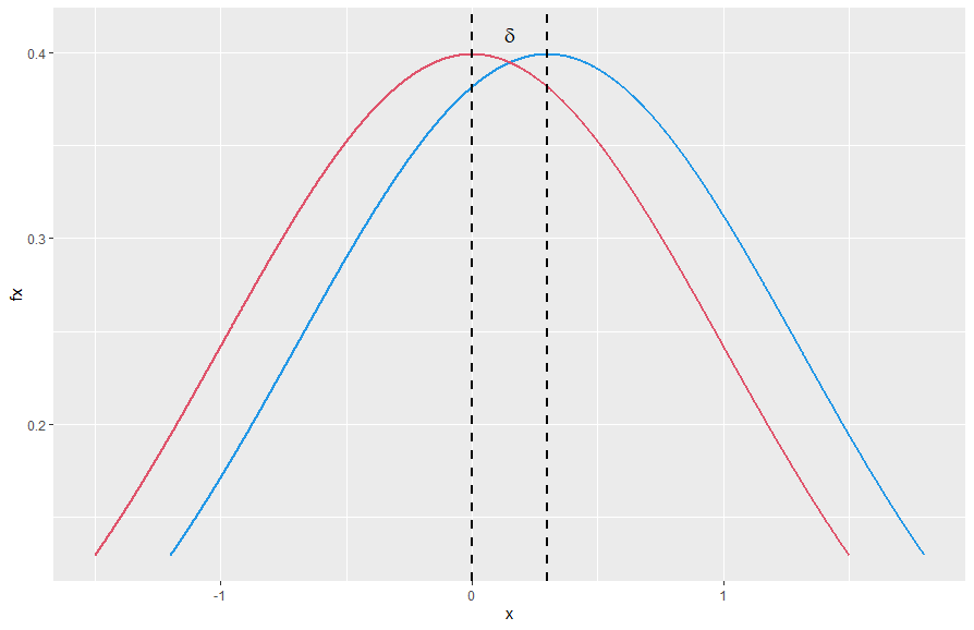
\[\frac{X}{s_p} \sim N\left(\frac{\mu_1}{s_p},1\right) ~\text{, }~\frac{Y}{s_p} \sim N\left(\frac{\mu_2}{s_p},1\right) ~\text{ and }~ \frac{X-Y}{s_p} \sim N\left(\delta,2\right).\]Then, we can plot their densities on the same graph as shown below. Here the blue one corresponds to the density of $X/s_p$ with center $\mu_1/s_p$ and the red one corresponds to the density of $Y/s_p$ with center $\mu_2/s_p$ and their centers are exactly $\delta$ units away from each other.
The overlapping coefficient (OVL) refers to the area under these two probability densities simultaneously. Note that this area is symmetric around the gray axis in the plot below. So we can compute it as follows:
\[\text{ OVL } = 2\Phi\left(\frac{\vert \delta\vert}{2}\right).\]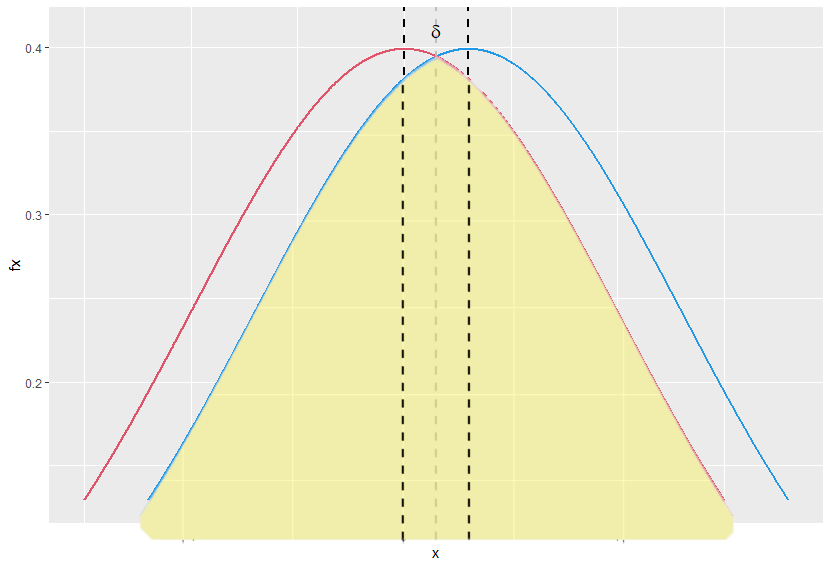
Probability of superiority is the probability that a randomly selected individual from the treatment group will have a higher score than a randomly selected individual from the control group, i.e., $P(X > Y)$. From our last observation above $\frac{X-Y}{s_p} \sim N\left(\delta,2\right)$, we know that
\[\frac{\frac{X-Y}{s_p} - \delta }{ \sqrt 2}\sim N\left(0,1\right).\]Thus,
\[P(X>Y) = P\left(\frac{\frac{X-Y}{s_p} - \delta }{ \sqrt 2}> -\frac{\delta}{\sqrt 2} \right) = P\left(Z > -\frac{\delta}{\sqrt 2}\right) = \Phi\left( \frac{\delta}{\sqrt 2}\right).\]Cohen’s $U_3$ is defined as the percentage of the control group’s population which the upper half of the cases of the treatment group’s population exceeds. It’s just the area in yellow as shown below. Clearly,
\[U_3 = \Phi(\delta).\]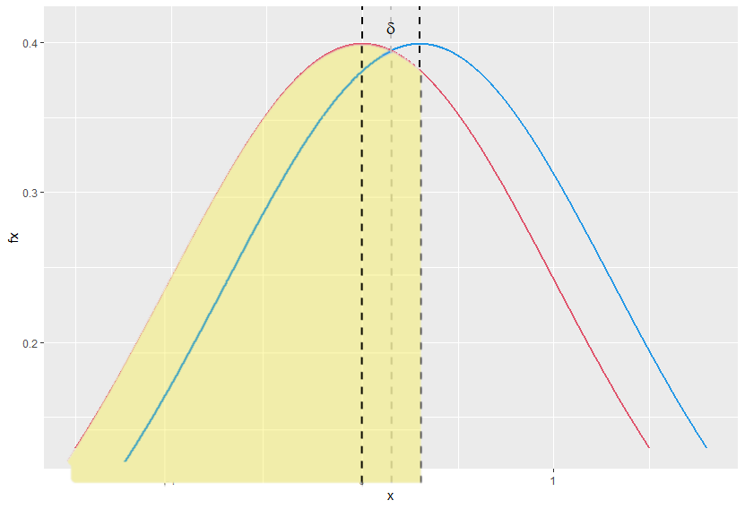
Q1. What can we do if the sample sizes are not large enough?
A1. Then, we can use the following fact:
\[T = \frac{\bar{X}-\bar Y}{s_p\sqrt{1/n+1/m}} \sim t_{(n+m-2)} \text{ under } H_0,\]Hint: Recall that if $U\sim N(0,1), V\sim\chi^2_{(r)}$ and $U$ is independent of $V$, then
\[\frac{U}{\sqrt{V/r}} \sim t_{(r)}.\]Q2. What if the two samples have unequal variances?
A2. See Welch’s t-test.