The following problem originates from one of my earlier post 11-or-12.
Suppose A and B play a game of fair dice. A keeps throwing the fair die until he obtains the sequence “11” in two successive throws. B throws the die until he obtains the sequence “12” in two successive throws.
We’ve found their expected waiting times. Now let’s try to derive the exact distribution of their waiting times.
Let’s compute the distribution of $X=[\text{ total number of throws until the first “11” }]$. We consider all possible states for every two successive throws in this process. There are four different states of our interest: $xx, 1x, x1$ and $11$, where $x$ denotes any number from \(\{2,3,4,5,6\}\). For example, a sequence of “16311” implies the states transitions: $1x \to xx \to x1 \to 11$. Next, we consider the transition probabilities between these states. For the state $xx$, we have:
\[P(xx \to xx) = P_{xx,xx} = \frac{5}{6},~P_{xx,1x} = 0,~P_{xx,x1} = \frac{1}{6} \text{ and }~P_{xx,11} =0.\]By similar argument, we obtain the following transition matrix:
\[P = \begin{pmatrix} \frac{5}{6} & 0 & \frac{1}{6} & 0 \\ \frac{5}{6} & 0 & \frac{1}{6} & 0 \\ 0 & \frac{5}{6} & 0 & \frac{1}{6} \\ 0 & 0 & 0 & 1 \end{pmatrix},\]where the order of the states are $xx, 1x, x1$ and $11$ for both row and column. Note that we make the state 11 an absorbing state.
Let $p_0 = (p_1,p_2,p_3,p_4)$ be the initial distribution. Then after $n$ steps, the state distribution is given by the vector $p_0P^n$, where the last entry of this vector is the probability of being in state 11 after $n$ steps. This is not exactly what we want. We need to change our entry $P_{4,4}$ from 1 to 0:
\[P_* = \begin{pmatrix} \frac{5}{6} & 0 & \frac{1}{6} & 0 \\ \frac{5}{6} & 0 & \frac{1}{6} & 0 \\ 0 & \frac{5}{6} & 0 & \frac{1}{6} \\ 0 & 0 & 0 & 0 \end{pmatrix},\]so that the last entry of the vector $p_0P_*^n$ is the probability that we are in state 11 after exactly $n$ steps.
Note that we have to roll the dice twice to determine our initial state. Therefore, the initial distribution $p_0 = (p_1,p_2,p_3,p_4)$ can be easily derived:
\[p_1 = p_{xx} = \frac{25}{36},~p_2 = p_{1x} = \frac{5}{36},~ p_3 = p_{x1} = \frac{5}{36}~\text{ and }~ p_4 = p_{11} = \frac{1}{36}.\]The last thing to note is that $X$ has a support \(\{2,3,\dots\}\) and the actual correspondence is:
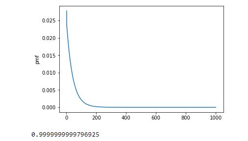
\[P(X = x) = (p_0P_*^{x-2})_4,\]where $(\cdot)_4$ means the fourth element of this vector. The following is the code in Python for plotting the first 1000 probability masses of $X$.
import numpy as np
import matplotlib.pyplot as plt

p0 = np.matrix( (25/36, 5/36, 5/36, 1/36) )
P = np.matrix( ((5/6, 0, 1/6, 0), (5/6, 0, 1/6, 0), (0, 5/6, 0, 1/6), (0, 0, 0, 0)) )
temp = p0
n = np.array([])
prob = np.array([])

# Compute and plot the first 1000 probabilities.
# Note that the support of this r.v. is 2,3,..., so n should range from 2 to 1002.
for i in range(1000):
    n = np.append(n, i+2)
    prob = np.append(prob, temp[0,3])
    temp = temp*P

plt.plot(n, prob)
plt.ylabel('pmf')

# Let's check if it's a legitimate pmf.
print(np.sum(prob))
Output is as follows:
Similarly, we may also determine the distribution of $Y=[\text{ total number of throws until the first “12”}]$ if we want.